Vertex operator algebra

In mathematics, a vertex operator algebra (VOA) is an algebraic structure that plays an important role in conformal field theory and related areas of physics. Vertex operator algebras have proven useful in purely mathematical contexts such as monstrous moonshine and the geometric Langlands correspondence.

Vertex operator algebras were first introduced by Richard Borcherds in 1986, motivated by the vertex operators arising from field insertions in two dimensional conformal field theory, a framework that is essential to define string theory. The axioms of a vertex operator algebra are a formal algebraic interpretation of what physicists called chiral algebras, whose definition was made mathematically rigorous by Alexander Beilinson and Vladimir Drinfel'd.

Important examples of vertex operator algebras include lattice VOAs (modeling lattice conformal field theories), VOAs given by representations of affine Kac-Moody algebras (from the WZW model), the Virasoro VOAs (i.e., VOAs corresponding to representations of the Virasoro algebra) and the moonshine module V^♮, constructed by Frenkel, Lepowsky and Meurman in 1988.

1 Formal definition
2 Symmetries
3 Motivation and related algebraic structures
4 Alternative definitions
5 Jacobi identity
6 A trivial example
7 Heisenberg Lie algebra example
8 Virasoro vertex operator algebra example
9 Monster Vertex Algebra
10 Vertex operator superalgebra
11 Vertex operator algebra defined by a lattice
- 11.1 Examples
12 Notes
13 References

Formal definition

A vertex algebra is a vector space V, together with an identity element 1∈V, an endomorphism T: V → V, and a linear multiplication map

$Y \colon V \otimes V \to V((z))$

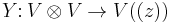
from the tensor product of V with itself to the space V((z)) of all formal Laurent series with coefficients in V, written as:

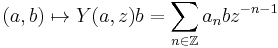
$(a, b) \mapsto Y(a,z)b = \sum_{n \in \mathbb{Z}} a_n b z^{-n-1}$

and satisfying the following axioms:

(Identity) For any a ∈ V,

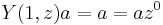$Y(1,z)a = a = az^0$ and $Y(a,z)1 \in a %2B zV[[z]]$
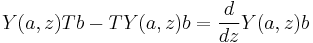
(Translation) T(1) = 0, and for any a, b ∈ V,

$Y(a,z)Tb - TY(a,z)b = \frac{d}{dz}Y(a,z)b$
(Four point function) For any a, b, c ∈ V, there is an element

$X(a,b,c;z,w) \in V[[z,w]][z^{-1}, w^{-1}, (z-w)^{-1}]$

such that Y(a,z)Y(b,w)c, Y(b,w)Y(a,z)c, and Y(Y(a,z-w)b,w)c are the expansions of X(a,b,c;z,w) in V((z))((w)), V((w))((z)), and V((w))((z-w)), respectively.

The multiplication map is often written as a state-field correspondence

$Y \colon V \to (\operatorname{End}\, V)[[z^{\pm 1}]]$

associating an operator-valued formal distribution (called a vertex operator) to each vector. Physically, the correspondence is an insertion at the origin, and T is a generator of infinitesimal translations. The four-point axiom combines associativity and commutativity, up to singularities. Note that the translation axiom implies Ta = a_-21, so T is determined by Y.

A vertex algebra V is Z₊-graded if

$V = \bigoplus_{n=0}^\infty V_n\,$

such that if a ∈ V_k and b ∈ V_m, then a_n b ∈ V_k+m-n-1.

A vertex operator algebra is a Z₊-graded vertex algebra equipped with a Virasoro element ω ∈ V₂, such that the vertex operator

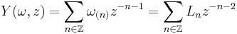
$Y(\omega, z) = \sum_{n\in\mathbb{Z}} \omega_{(n)} {z^{-n-1}} = \sum_{n\in\mathbb{Z}} L_n z^{-n-2}$

satisfies for any a ∈ V_n, the relations:

$L_0 a = na$
$Y(L_{-1} a, z) = \frac{d}{dz} Y(a, z) = [Y(a,z),T]$
$[L_m, L_n]a = (m - n)L_{m %2B n}a %2B \delta_{m %2B n, 0} \frac{m^3-m}{12}ca$

where c is a constant called the central charge, or rank of V. In particular, this gives V the structure of a representation of the Virasoro algebra.

Symmetries

The reason for the translation operator, T, and the Virasoro operators, L, come from the idea that we are interested in systems with translational and 2D conformal symmetries respectively. (With both these symmetries the system will also have rotational and scale invariance also.)

Motivation and related algebraic structures

The axioms of a vertex algebra are obtained from abstracting away the essentials of the operator product expansion of operators in a 2D Euclidean chiral conformal field theory. The two dimensional Euclidean space is treated as a Riemann sphere with the point at infinity removed. V is taken to be the space of all operators at $z=0$ . The operator product expansion is holomorphic in z and so, we can make a Laurent expansion of it. 1 is the identity operator. We treat an operator valued holomorphic map over $\mathbb{C} \setminus \{0\}$ as a formal Laurent series. This is denoted by the notation V((z)). A holomorphic map over $\mathbb{C}$ is given by a Taylor series and as a formal power series, this is denoted by V[[z]].

The operator b(0) is abstracted to b and the operator a(z) to Y(a,z). The derivative a'(z) is abstracted to -Ta.

If one considers only the singular part of the OPE in a Vertex algebra, one arrives at the definition of a Lie conformal algebra. Since one is often only concerned with the singular part of the OPE, this makes Lie conformal algebras a natural object to study.

Alternative definitions

Another way to think of vertex algebras is as a generalisation of a Lie algebra with the addition of a continuous variable to both the generators of the algebra and the structure constant. (The structure constants define the algebra). So we would have:

$\lambda^A(x) \otimes \lambda^B(y) = f^{A,B,C}(x) \lambda_C (y)$

which can also be expressed without the y dependence as:

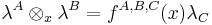
$\lambda^A \otimes_x \lambda^B = f^{A,B,C}(x) \lambda_C$

which reveals the Vertex Multiplication as a group operation in which the group constants vary with their position on the conformal sheet.

Jacobi identity

The vertex algebras satisfy a generalisation of the Jacobi identity given by:

$z^{-1}\delta\left(\frac{y-x}{z}\right)Y\left(a,x\right)Y(b,y)c - z^{-1}\delta\left(\frac{-y%2Bx}{z}\right)Y(b,y)Y(a,x)c = y^{-1}\delta\left(\frac{x%2Bz}{y}\right)Y(Y(a,z)b,y)c$

which can also be written as

$z^{-1}\delta\left(\frac{y-x}{z}\right) (a \otimes_x(b \otimes_y c)) - z^{-1}\delta\left(\frac{-y%2Bx}{z}\right)(b \otimes_y(a \otimes_x c)) = y^{-1}\delta\left(\frac{x%2Bz}{y}\right)((a\otimes_z b)\otimes_y c)$

where the delta function is defined formally by:

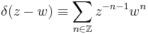
$\delta(z-w) \equiv \sum_{n \in \mathbb{Z}} z^{-n-1}w^n$

(always expanded in terms of the second variable w)

A trivial example

To make things more concrete a trivial example of a commutative vertex algebra is presented. We take the vector space V to consist of 2-vectors, v, with components $v=(p,q)^T$ . If we think of this vector as a complex number, p+qi, the Y function can be seen as taking it from its vector form to a 2x2 matrix form of (p-qz)+qi. The p and q are real numbers.

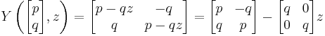
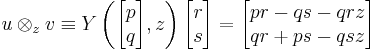
$Y\left(\begin{bmatrix} p \\ q \end{bmatrix},z\right) = \begin{bmatrix} p-qz & -q \\ q & p-qz \end{bmatrix} = \begin{bmatrix} p & -q \\ q & p \end{bmatrix} - \begin{bmatrix} q & 0 \\ 0 & q \end{bmatrix} z$

So that multiplication between two vectors $u=(p,q)^T$ and $v=(r,s)^T$ is defined by:

$u\otimes_z v \equiv Y\left(\begin{bmatrix} p \\ q \end{bmatrix},z\right)\begin{bmatrix} r \\ s \end{bmatrix} = \begin{bmatrix} pr-qs - qrz \\ qr%2Bps -qsz \end{bmatrix}$

The identity element 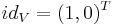$id_V = (1,0)^T$ so that:

$Y\left( \begin{bmatrix} 1 \\ 0 \end{bmatrix},z\right) = \begin{bmatrix} 1 & 0 \\ 0 & 1 \end{bmatrix}$

and

$Y\left( \begin{bmatrix} p \\ q \end{bmatrix},z\right)\begin{bmatrix} 1 \\ 0 \end{bmatrix} = \begin{bmatrix} p \\ q \end{bmatrix} %2B O(z)$

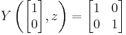
and the operator T in this example is:

$T = \begin{bmatrix} 0 & 1 \\ 0 & 0 \end{bmatrix}$

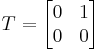
it is easy to check:

$\frac{d}{dz} \begin{bmatrix} p-qz & -q \\ q & p-qz \end{bmatrix} = \begin{bmatrix} 0 & 1 \\ 0 & 0 \end{bmatrix} \begin{bmatrix} p-qz & -q \\ q & p-qz \end{bmatrix} - \begin{bmatrix} p-qz & -q \\ q & p-qz \end{bmatrix} \begin{bmatrix} 0 & 1 \\ 0 & 0 \end{bmatrix}$

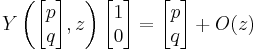
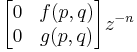
Since the Y matrices commute, locality is satisfied trivially. Non-trivial vertex algebras and vertex operator algebras would require infinite sized matrices to represent them. All the terms with powers of $z^n$ with n<0 must be zero when applied to the identity vector $id_V$ . i.e. of the form:

$\begin{bmatrix} 0 & f(p,q) \\ 0 & g(p,q) \end{bmatrix} z^{-n}$

but adding a single term like this won't commute with the other terms. Hence our example would no longer be trivial since we may need an infinite number of terms to restore locality.

Heisenberg Lie algebra example

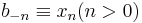
The Heisenberg Lie algebra is defined by the commutation relations:

$[b_n,b_m]=n \delta_{n,-m}$

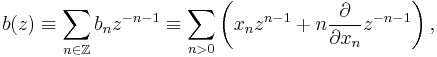
One representation is to define the operators b, in terms of the dummy variables x as:

$b_{-n} \equiv x_n (n>0)$

$b_n \equiv n \frac{\partial}{\partial x_n} (n<0)$

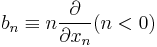
and $b_0=0$ .

This can be made into a vertex algebra by the definition:

$Y( x_{n_1%2B1}x_{n_2%2B1}x_{n_3%2B1}...x_{n_k%2B1}, z) \equiv \frac{1}{n_1!n_2!..n_k!}:\partial^{n_1}b(z)\partial^{n_2}b(z)...\partial^{n_k}b(z):$

where :..: denotes normal ordering (i.e. moving all derivatives in x to the right). Thus Y(1,z) = Id.

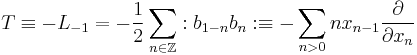
T is defined by the conditions T.1 = 0 and

$[T,b_n] = -nb_{n-1}.$

Setting

$b(z) \equiv \sum_{n \in \mathbb{Z}} b_n z^{-n-1} \equiv \sum_{n>0} \left( x_n z^{n-1} %2B n \frac{\partial}{\partial x_n } z^{-n-1} \right),$

it follows that

$L(z)\equiv \sum_{n\in \Bbb Z} L_n z^{-n-2}={1\over 2}�:b(z)^2:$

and hence:

$T \equiv -L_{-1}=-{1\over 2} \sum_{n \in \mathbb{Z}}�:b_{1-n}b_n: \equiv - \sum_{n>0} n x_{n-1} \frac{\partial}{\partial x_n}$

The vertex operators may also be written as a functional of a multivariable function f as:

$Y[f,z] \equiv�:f(\frac{b(z)}{0!},\frac{b'(z)}{1!},\frac{b''(z)}{2!},...):$

if we understand that each term in the expansion of f is normal ordered.

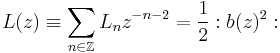
Virasoro vertex operator algebra example

The Virasoro vertex operator algebra is a conformal vertex algebra. It is defined as follows:

$Y(L_{-n_1-2}L_{-n_2-2}...L_{-n_k-2}|0\rangle,z) \equiv \frac{1}{n_1!n_2!..n_k!}:\partial^{n_1}L(z)\partial^{n_2}L(z)...\partial^{n_k}L(z):$

With L(z) defined as above. So we have $id_V = |0\ran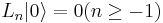gle$ and with $L_n|0\rangle = 0 (n\ge -1)$ and $\omega = L_{-2}|0\rangle$ . We see that this satisfies the axioms of a vertex algebra and includes a representation of the Virasoro algebra. The fact that the Virasoro field $L(z)$ is local can be deduced from the formula for its self-commutator:

$[L(z),L(w)] =\left(\frac{\partial}{\partial w}L(w)\right)w^{-1}\delta \left(\frac{z}{w}\right)-2L(w)w^{-1}\frac{\partial}{\partial z}\delta \left(\frac{z}{w}\right)-\frac{1}{12}cw^{-1}\left(\frac{\partial}{\partial z}\right)^3\delta \left(\frac{z}{w}\right)$

where c is central charge.

Monster Vertex Algebra

The monster vertex algebra is a conformal vertex operator derived from 26 dimensional bosonic string theory compactified on the hyper-torus induced by the Leech lattice and orbifolded by the two-element reflection group. It is denoted as $V^\natural$ . It was used to prove the Monstrous moonshine conjectures.

In the string model the vectors a in Y(a,z) are the different states or vibrational modes of the string which correspond to different particles and polarisations and z is a point (or vertex) on the world sheet which corresponds to an ingoing or outgoing string. Hence why it is called a Vertex Algebra.

Vertex operator superalgebra

When the underlying vector space V has a Z₂ grading, so that it splits as a sum of even and odd parts

$V=V_%2B\oplus V_-$

with 1 in V₊, the structure of a vertex superalgebra can be defined on V by incorporating the usual rule of signs in the axiom for the four point function:

(Four point function) For any a, b, c ∈ V_±, there is an element

$X(a,b,c;z,w) \in V[[z,w]][z^{-1}, w^{-1}, (z-w)^{-1}]$

such that Y(a,z)Y(b,w)c, εY(b,w)Y(a,z)c, and Y(Y(a,z-w)b,w)c are the expansions of X(a,b,c;z,w) in V((z))((w)), V((w))((z)), and V((w))((z-w)), respectively, where ε is -1 if both a and b are odd and 1 otherwise.

If in addition there is a Virasoro element ω in the even part of V₂, then V is called a vertex operator superalgebra. One of the simplest examples is the vertex operator superalgebra generated by a single complex fermion.^[1]

Vertex operator algebra defined by a lattice

Let Λ be an integral lattice in Euclidean space X = R^N, i.e. a subgroup isomorphic to Zⁿ with m ≤ N and such that (α,β) lies in Z for α,β in Λ . The lattice is said to be even if (α,α) is even for each α in Λ. Setting

$\displaystyle{B(\alpha,\beta)=(-1)^{(\alpha,\beta)}}$

there is an essentially unique normalised cocycle ε(α,β) with values ±1 such that

$B(\alpha,\beta)=\varepsilon(\alpha,\beta)\varepsilon(\beta,\alpha).$

and the cocycle identity

$\varepsilon(\alpha%2B\beta,\gamma)\varepsilon(\alpha,\beta)=\varepsilon(\alpha,\beta%2B\gamma)\varepsilon(\beta,\gamma)$

is satisfied along with the normalisation conditions

$\varepsilon(\alpha,-\alpha)=\varepsilon(\alpha,0)=\varepsilon(0,\alpha)=1.$

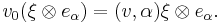
A cocycle representation can be defined on C[Λ], with basis e_α (α in Λ), by

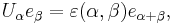
$U_\alpha e_\beta= \varepsilon(\alpha,\beta)e_{\alpha%2B\beta},$

Thus

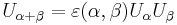
$\displaystyle{U_{\alpha%2B\beta}=\varepsilon(\alpha,\beta) U_\alpha U_\beta}$

and

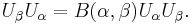
$\displaystyle{U_\beta U_\alpha =B(\alpha,\beta) U_\alpha U_\beta.}$

The operators U_α are unitary if the e_α are taken to be orthonormal.

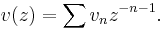
There is a bosonic system associated to X, namely operators v_n depending linearly on v in X such that

$\displaystyle{[v_m,u_n]=m(v,u)\delta_{m%2Bn,0}I.}$

In addition the system has a derivation D satisfying with

$\displaystyle{[D,v_n]=-nv_n.}$

There is a unique irreducible representation of this system characterised by the existence of a vacuum vector Ω with v_n Ω = 0 for n ≥ 0. The underlying space S has a unique inner product structure for which v_n* = v_–n. The vector space V of the vertex superalgebra is defined by

$V =S \otimes {\Bbb C}[\Lambda]=\bigoplus_{\alpha \in \Lambda} S \otimes e_\alpha.$

The operators v_n with n non-zero act on $S\otimes e_\alpha$ exactly as they act on S,

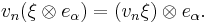
$v_n(\xi\otimes e_\alpha)=(v_n\xi)\otimes e_\alpha.$

The operators v₀ act as scalars on $S\otimes e_\alpha$ :

$v_0(\xi\otimes e_\alpha)=(v,\alpha) \xi \otimes e_\alpha.$

For each v in X define the field

$v(z)=\sum v_n z^{-n-1}.$

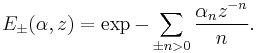
For each α in Λ define

$\Phi_\alpha(z)=U_\alpha z^{\alpha_0} E_-(\alpha,z)E_%2B(\alpha,z),$

where

$E_\pm(\alpha,z) =\exp -\sum_{\pm n>0} {\alpha_n z^{-n} \over n}.$

If v⁽ⁱ⁾ is an orthonormal basis of X, define

$L(z)\equiv \sum L_n z^{-n-2} = {1\over 2} \sum_i�: v^{(i)}(z)^2:$

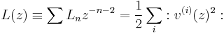
where the normal ordering is given by

$�:v(z)^2:= \sum_{n<0} v_n z^{-n-1} v(z) %2B v(z)\sum_{n\ge 0} v_n z^{-n-1}.$

Then the vertex operators v(z) and Φ_α(z) generate a vertex operator superalgebra with underlying space V. The operators D and T are given by L₀ and L_–1 respectively.^[2]^[3]

Examples

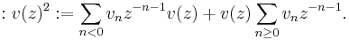
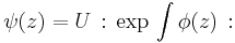
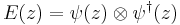
The lattice Z in R gives the vertex operator superalgebra corresponding to a single complex fermion. This is another way of phrasing the celebrated fermion-boson correspondence. The fermion field ψ(z) and its conjugate field ψ^†(z) are defined by

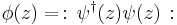
$\psi(z)=\sum e_nz^{-n-1},\,\,\, \psi^\dagger(z)=\sum e_n^*z^n,\,\,\,\{e_n,e_m\}=0,\,\,\,\{e_m,e_n^*\}=\delta_{m,n}I.$

The correspondence between fermions and a single charged boson field

$\phi(z)=\sum a_nz^{-n-1},\,\,\, [a_m,a_n]=m\delta_{n%2Bm,0}I,\,\, Ua_nU^{-1}=a_n - \delta_{n,0}I$

takes the form

$\phi(z)=\,:\,\psi^\dagger(z)\psi(z)\,:$

$\psi(z)=U \,:\,\exp \, \int \phi(z) \,:$

where the normal ordered exponential is interpreted as a vertex operator of the type constructed above.

The lattice √2 Z in R gives the vertex operator algebra corresponding to the affine Kac-Moody algebra $\widehat{sl(2)}$ at level one. It is realised by the fields

$H(z)=\phi(z)\otimes I - I\otimes \phi(z)$

$E(z)=\psi(z)\otimes \psi^\dagger(z)$

$F(z)=\psi^\dagger(z)\otimes \psi(z)$

If Λ is even, is generated by its "root vectors" (those satisfying (α,α)=2), spans X, and any two root vectors are joined by a chain of root vectors with consecutive inner products non-zero then the vertex operator algebra corresponds to the affine Kac-Moody algebra of a simply laced simple Lie algebra at level one. The zero modes of the v(z)'s and the Φ_α(z)'s corresponding to root vectors give a construction of the underlying simple Lie algebra, related to a presentation originally due to Jacques Tits. The definition of the vertex operators Φ_α(z) in this context is originally due to Victor Kac, Igor Frenkel and independently Graeme Segal.^[4]^[5] It is based on the earlier construction by Sergio Fubini and Gabriele Veneziano of the tachyonic vertex operator in the dual resonance model.

References

Borcherds, Richard (1986), "Vertex algebras, Kac-Moody algebras, and the Monster", Proc. Natl. Acad. Sci. USA. 83: 3068–3071
Frenkel, Igor; Lepowsky, James; Meurman, Arne (1988), Vertex operator algebras and the Monster, Pure and Applied Mathematics, 134, Academic Press, ISBN 0-12-267065-5
Kac, Victor (1998), Vertex algebras for beginners, University Lecture Series, 10 (2nd ed.), American Mathematical Society, ISBN 0-8218-1396-X
Frenkel, Edward; Ben-Zvi, David (2001), Vertex algebras and Algebraic Curves, Mathematical Surveys and Monographs, American Mathematical Society, ISBN 0-8218-2894-0
Xu, Xiaoping (1998), Introduction to vertex operator superalgebras and their modules, Springer, ISBN 0792352424